Scaling Monosemanticity on a Small LLaMA (and What Broke Along the Way)

What I Was Trying To Do

The high-level idea was simple:

1. Run a LLaMA model on a large text stream.
2. Save activations from a middle layer, per token.
3. Train a sparse autoencoder (SAE) to reconstruct those activations.
4. Treat the sparse latents as “features,” then inspect and steer them.

In practice, that means you are not asking “which neuron means X?” You are asking: can a learned sparse basis make features more legible than single neurons, and can you intervene on those features at inference time?

That was the bet.

The Actual Setup (Verified)

• Base model: meta-llama/Llama-3.2-3B.
• Activations: middle-layer activations, around layer 15 or 16.
• Hidden size: 3072.
• SAE: one hidden layer, ReLU, overcomplete width 2^16 = 65536.
• Data: streamed from monology/pile-uncopyrighted.
• Each activation row saved: per token with metadata for reverse lookup (sentence id, token index, token id).

If you want one sentence: we trained an SAE on token-level LLaMA activations and built a full inspection loop to retrieve top-activating contexts and manipulate features.

The First Real Lesson: Retrieval Is the Instrument

I learned this the hard way. If you cannot map an activation back to the exact token and its context, you do not have interpretability. You have numbers.

Saving token ids, sentence ids, and positions was not a logging detail. It was part of the scientific apparatus.

This shaped everything else: file layout, memory budget, batch sizes, and the way I wrote the activation extraction code.

What Worked (and Was Actually Exciting)

1. Interpretable features showed up early

Even with a modest model and a relatively straightforward SAE, features popped out that were clearly meaningful:

• medical and scientific writing
• emotions (positive vs negative)
• language and multilingual patterns
• AI and programming domains
• gender-bias artifacts

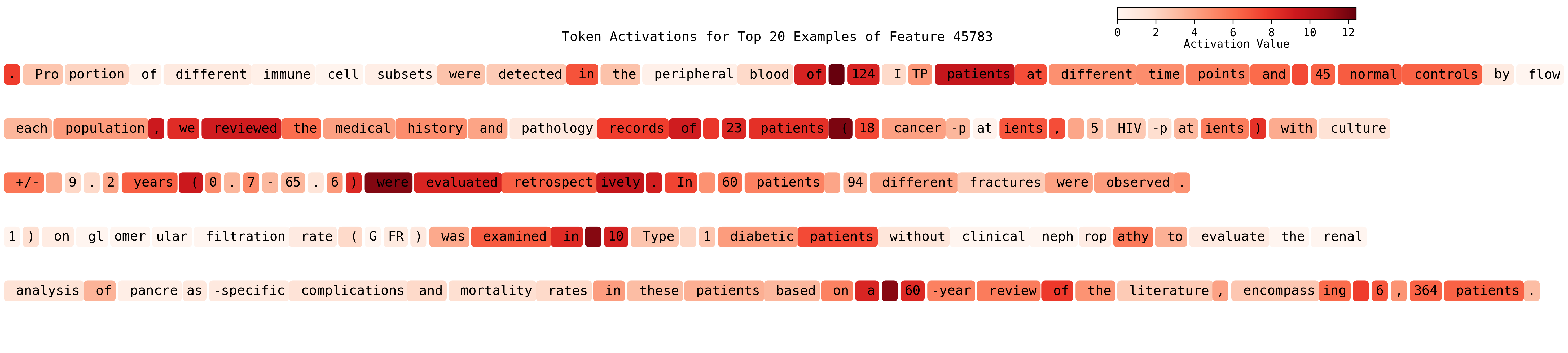
This alone was a big win. It suggested you don’t need frontier-scale models to get some interpretability traction. Concretely, a “medical/clinical” feature would spike on fragments like “patients were randomized,” “clinical trial,” “diagnosed with,” “mg/kg,” or “double-blind,” and the top-activating contexts looked exactly like paper abstracts and methods sections.

2. Some features were genuinely steerable

Once you can isolate a feature, you can try boosting it at inference. If that sentence is opaque, here is the operational version: you take the hidden activation vector at a layer, add a scaled version of a single SAE feature to it via the SAE decoder, and then let the model continue the forward pass. That is literally “turning the knob” on one learned feature direction.

That was the most compelling part of the project. A bias-related feature, when boosted, made stereotyped role assignments show up more often in completions (e.g., woman=nurse, man=doctor). A “medical” feature pushed the model into clinical-sounding continuations, like switching from “I am a student…” to something that starts talking about diagnoses, patients, trials, or treatment language. It is not deterministic, but the distribution visibly shifts.

That does not prove clean monosemanticity. But it does show a causal knob, which is stronger evidence than pure correlation.

3. Some features were language-independent, others language-specific

One fun qualitative result: a medical feature lit up across English and Spanish. At the same time, there were distinct features that seemed mostly language-specific, especially Spanish or French.

That is exactly the kind of mixed behavior you’d expect if the features are partially semantic and partially surface-form driven. In practice, a multilingual “medical” feature might activate on English and Spanish clinical text, while a language feature lights up on grammar and function words unique to one language.

What Was Actually Hard

1. Sparsity is fragile, boring, and hard to debug

Most failures looked like this:

• near-zero activations (collapsed sparsity)
• dead features
• sparse-looking features that were really just punctuation or scaffolding
• metrics that looked okay until they were inspected carefully

You can get apparent sparsity without meaningful decomposition. ReLU already creates zeros. That is not the same thing as useful sparsity.

The “boring” version looks like a feature that fires on commas, “the,” or line breaks, because those are everywhere and easy to compress.

A lot of time went into fixing loss formulas, sanity-checking the active-feature percentage, and tuning l1_lambda with much smaller changes than I expected.

2. High-frequency patterns dominate unless you fight them

A naive SAE will happily spend its capacity on:

• punctuation
• frequent articles
• boilerplate phrasing

This doesn’t mean the method is wrong. It means you need to actively shape the data distribution and maybe the layer choice. Stratified sampling and higher-layer activations seem like obvious next steps. Otherwise, your dictionary fills up with “grammar scaffolding” before it gets to concepts you actually care about.

3. Tooling details changed qualitative results

One of the more annoying surprises: same family of model weights, wildly different behavior depending on how they were loaded.

The base model from Hugging Face gave poor feature explanations. The instruct version worked much better for automated labeling. That is not a subtle difference. It is the kind that can invalidate your entire “feature interpretation” loop if you do not notice it.

For example, an LLM-based “feature naming” pass went from nonsense fragments to coherent labels once we switched variants. (Yes, we used a separate LLM to help label/name features; it’s a practical shortcut, not a ground-truth oracle.)

4. A data pipeline bug distorted my conclusions

At one point, validation was loading full activation files (~81k vectors) instead of respecting batch size. That made it look like batch size didn’t matter. It did. The pipeline was just bypassing it.

Lesson: before you interpret a hyperparameter effect, verify that the data path actually uses it. In this case, batch size appeared irrelevant because validation loaded an entire activation file at once, bypassing the batch settings entirely.

The HPC Detour

Once the experiments got large enough, I moved the pipeline onto HPC. The surprising part was not the GPU run itself, but the monitoring.

I ended up building a minimal monitoring stack inside the job:

• Node Exporter (CPU)
• NVIDIA DCGM Exporter (GPU)
• Prometheus (metrics)
• Grafana (dashboards)

It sounds like overkill until you’ve lost a 48-hour job to silent OOMs. After that, the dashboards are worth it. You can see GPU utilization, CPU saturation, and memory spikes in real time instead of guessing from logs.

The Honest Version of the Result

I did not reproduce Anthropic’s scale or guarantees. I did build an end-to-end sparse-feature pipeline on a smaller open model, and I got qualitative, steerable features with clear interpretability value.

That is a real result. But the work wasn’t about one magical model. It was about everything around it: retrieval, data indexing, loss debugging, sampling, monitoring.

If I had to compress the lesson into one line:

After a certain point, interpretability stops being a modeling problem and becomes a systems problem.

What I’d Do Next

If I were starting over, I’d do these earlier:

• Build retrieval and metadata storage before any training.
• Test top-k or switch SAE variants instead of only vanilla ReLU SAEs.
• Stratify sampling to avoid frequency domination.
• Move to HPC earlier, and monitor from day one.

Final Take

Sparse features are real enough to be useful, but not clean enough to be romantic about. The pipeline can surface meaningful structure, but it fails in boring, subtle, engineering ways before it succeeds.

That is the takeaway I wish I had at the beginning.